The Two Lines of Code That Simulate the Solar System

I just watched a video about orbital mechanics that broke my brain in the best way possible, and I can’t stop thinking about it.

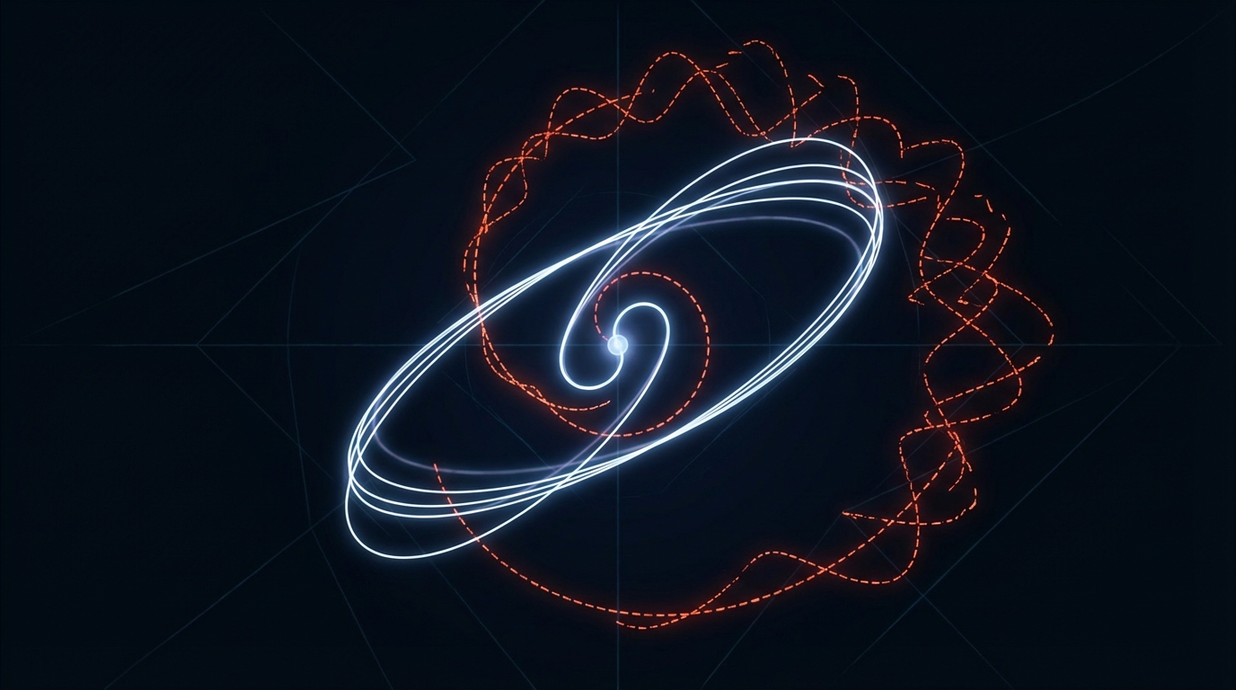
The setup seems simple enough - you want to simulate an asteroid orbiting the sun, you know Newton’s laws, and you write the obvious code: update position based on velocity, update velocity based on acceleration, run it. The orbit spirals outward, your asteroid escapes into the void, and the simulation breaks.

This isn’t a bug in your math - it’s a fundamental problem with how you’re stepping through time. For decades, this meant that simulating orbital dynamics over millions of years was essentially impossible, not because computers were too slow, but because the algorithms themselves became unstable long before reaching those timescales.

Then in 1991, astrophysicists borrowed an idea from molecular dynamics and everything changed - the fix was to swap two lines of code.

The Problem Everyone Was Getting Wrong

Here’s the naive approach: you have position and velocity, and at each time step you update position using the current velocity and then update velocity using the current acceleration. Both updates use the “old” values, which makes sense given what the equations suggest.

Run it and the orbit spirals outward; make your time steps smaller and it spirals slower, but it still spirals because the error accumulates. Given enough time, your simulation explodes.

Now swap the order - update velocity using the current acceleration first, and then update position using the new velocity. Same calculations, different order, with the second line now using the freshly updated velocity instead of the old one.

Run it and the orbit stays stable, not just for thousands of years but for billions of orbits with the error staying below 10^-10, practically machine precision. This isn’t just a different spiral - it’s qualitatively different behavior where the simulation that was fundamentally broken is now fundamentally stable.

Why Swapping Lines Changes Everything

The answer lives in phase space.

Normal space tracks where objects are located, but phase space tracks both location AND velocity simultaneously. For a particle moving in one dimension, phase space is two-dimensional with position on one axis and velocity on the other.

Here’s the key insight - when particles move according to Newton’s laws, they don’t just trace paths through phase space, they preserve certain geometric properties as they go, specifically area.

Imagine a cloud of particles in phase space where each represents a slightly different starting condition. As time passes, that cloud shears and stretches and deforms, but its total area never changes. This is Liouville’s theorem, a fundamental truth about how classical mechanics works.

The naive algorithm violates this at each step where the phase space area grows slightly and those tiny violations accumulate until eventually your simulation bears no resemblance to reality. The swapped algorithm preserves area exactly - each step is a shearing motion where the shape distorts but the area stays constant. You can run it forever and the fundamental geometry stays intact.

The 1991 Breakthrough

This principle, called symplectic integration, had been used in molecular dynamics since the 1960s, but in 1991 astrophysicists Jack Wisdom and Matthew Holman transformed it into a breakthrough for planetary simulation.

The Wisdom-Holman integrator took this area-preserving property and combined it with a key insight about orbital mechanics: most of the motion is just Keplerian orbits around the sun, with small perturbations from other planets.

For pure Keplerian motion, you can solve the equations exactly with no approximation needed, so instead of approximating everything, you solve the dominant motion exactly and only approximate the small perturbations. This lets you take massive time steps where previous methods might need millions of steps per orbit while this approach can take just a handful, and because it preserves the geometric structure of the dynamics, it stays stable over astronomical timescales.

The Kirkwood Gaps

The payoff was immediate.

The asteroid belt between Mars and Jupiter has a striking feature where certain orbital distances are almost empty - these are the Kirkwood gaps, noticed by astronomers for over 150 years.

The gaps appear at orbital distances where asteroids would orbit the sun a small-integer number of times for each Jupiter orbit, and these resonances create gravitational chaos. Over millions of years, asteroids get ejected from these regions.

Before symplectic integration, you couldn’t simulate this because the algorithms broke down long before the gaps would emerge. After? Scientists could finally watch the gaps form in their simulations, matching what we see in the real asteroid belt.

Two Lines

What gets me about this story is how small the change looks and how profound the consequences are.

Two lines of code, swapped, and the difference between a simulation that self-destructs and one that runs for a billion years.

It’s not about being clever with approximations or using fancier math - it’s about respecting the underlying geometry of the physics. The universe preserves phase space area, and if your algorithm doesn’t, you’re fighting against reality itself.

There’s a beauty to that. The best numerical methods aren’t brute-force approximations, they’re the ones that preserve what the physics says should be preserved with the geometry of motion baked into the algorithm.

I keep wondering what else works this way, what other problems we’ve been attacking head-on when the real solution is respecting some deeper structure we didn’t know was there.

The solar system runs on rules, and the code that simulates it works best when it follows those same rules - not just approximately, but exactly, at the geometric level.

Two lines swapped - that’s the difference between chaos and a solar system.

Source: The Code That Revolutionized Orbital Simulation by Brainuffle